VLOOKUP – explained once and for all

I consider being able to use the Vlookup function, as easily as you were writing your name, to be a key part of graduating from ‘Excel user’ to ‘Excel guru’ status.

Microsoft explains;

“Use VLOOKUP, one of the lookup and reference functions, when you need to find things in a table or a range by row.”

 

Now all credit to Microsoft and their support section, I truly find it very useful for the most part, but that really isn’t a clear enough explanation to me. For me, the first step to learning is to understand what you are trying to achieve and why you need it in the first place.

I would say;

“VLOOKUP is used to bring relevant information from one range of cells to another.”

 

In essence, you can use VLOOKUP to look through a list, find the piece of information that you need, bring it back to the sheet or cells that you need it in, and put it in the right place. Magic!

Like everything in life, and Excel, there are a couple of limitations to how you can use this great power:

1. Your data has to be in a reasonably clean state. That means a separate row for each different product, item, person, location or whatever you have in your list.
2. You need a unique identifier, this is something in each row that refers to that entry only, a product code, an employee number, a Postal/Zip code etc.
3. VLOOKUP is short for Vertical LOOKUP and it works from left to right, the range you are looking into must be arranged with the unique identifier somewhere to the left of the data you want to bring back.

 

 

Let’s get to the formula, then break it down bit by bit. Be warned, I am going to say ‘unique identifier’ an awful lot!

=vlookup(this value, in this list, and get me value in this column, approx. or exact match?)

 

=vlookup(

This tells Excel that you are using a function, the equals sign tells it that it should check its functions for the next bit of text (Vlookup in this case) to check the rules of what it should do next. Most of Excel’s functions need some input to work and the brackets are where it looks for these.

this value

This is your unique identifier, something that is found in both locations, where you are looking for the information, and where you are bringing it back to. You can either type it in double quotations “this text”, or reference a cell that has this unique identifier in. Best practice is to reference a cell as this will let you fill the formula down, and each subsequent formula will be working bring back a different result.

in this list

This is where Excel should look for the data, this is a range of cells that includes both the unique identifier and the result you are looking for. In most cases, the best approach is to select full columns instead of a range of x rows and x columns, this way you don’t have to worry about absolute and relative references when you are copying your formula down in your original sheet, the range always stays the same.

and get me a value in this column

This is the number of columns away your unique identifier is from the piece of data you want, inclusive of both the unique identifier’s column and the desired data’s column. So for example, if you are looking from column A to D, you would enter 4 here.

approx. or exact match?)

There are times when you want to match your unique identifiers exactly, (a name, product code, postal/zip code) and there are times when pretty close is good enough, (a number that runs to 20 decimal points). If you want exact match enter FALSE, if you want an approximate enter TRUE. Simple. This is generally the most confusing part of the whole thing. 

Lastly, close off the brackets to let Excel know that the function is complete. Like in all functions, each piece (argument) is separated by a comma.

 

In this example, I have used the same sheet for clarity, this could easily be used across multiple sheets or even workbooks. The only difference you will see is the range references change to include the worksheet name or workbook name (and path) if you are doing this, but the process remains the same.

Here we have two lists, some information I have recorded myself, and a list of general information. I want to combine these two into one list of information. In E2 I enter the formula:

=VLOOKUP(A2,G:H,2,FALSE)

 

 

Top tip: You can use just your keyboard to type in the whole thing (and I encourage learning keyboard shortcuts to help you to be more productive!), but it is a lot more intuitive to use the mouse here.

 

 

 

And the missing piece of information is added to my first concise list. You can now fill this formula down and the function will adjust for each row and bring back the relative data. 

 

 

Find more quick tips like this and more on my post: Top skills to make you look like a wizard!

 

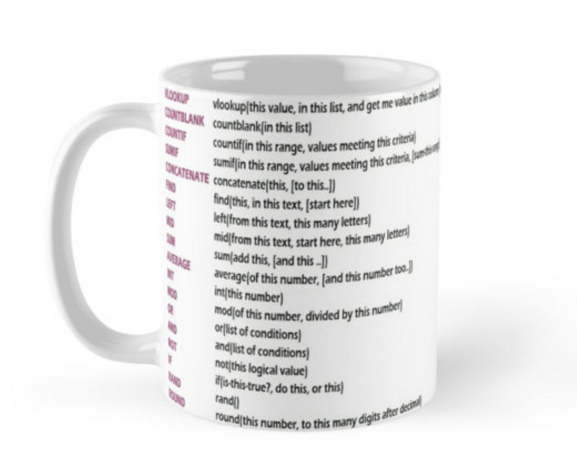
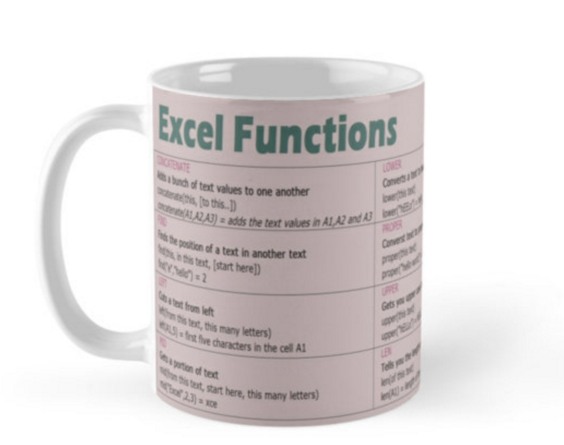
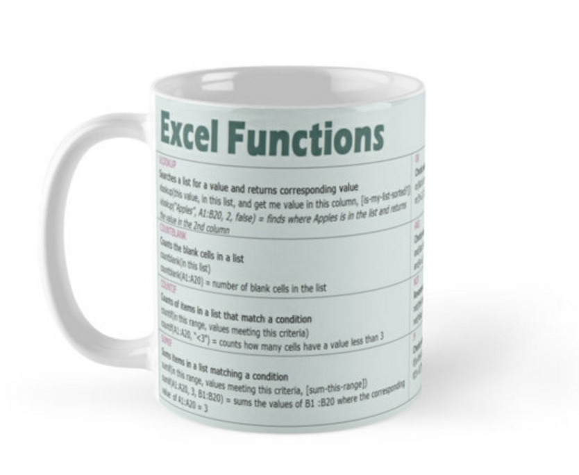
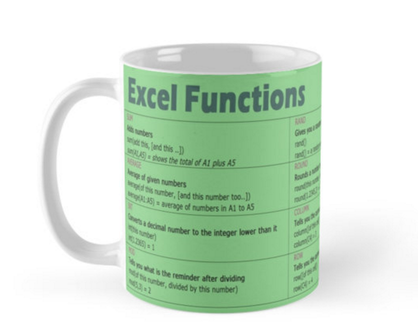
The Excel cheat sheet mugs below will give you a head start to becoming a Spreadsheet wizard!